Samvit Jain's blog

A Brief Primer: Stochastic Gradient Descent

20 Jul 2017

“Nearly all of deep learning is powered by one very important algorithm: stochastic gradient descent.” - Ian Goodfellow

Many machine learning papers reference various flavors of stochastic gradient descent (SGD) - parallel SGD, asynchronous SGD, lock-free parallel SGD, and even distributed synchronous SGD, to name a few.

This topic isn’t just a theoretical curiosity. Parallelizing important optimization algorithms, like SGD, is the key to fast training and, by extension, fast model development. Not surprisingly, three out of the four papers I just referenced came out of industry research.

To orient a discussion of these papers, I thought it would be useful to dedicate one blog post to briefly developing stochastic gradient descent from “first principles.” This discussion is supposed to be illustrative, and errs in favor of pedagogical clarity, over mathematical rigor.

Optimization

Stochastic gradient descent is an optimization algorithm. In machine learning, what exactly does an optimization algorithm optimize?

As you may know, supervised machine learning generally consists of two phases:¹ training (generating a model) and inference (making predictions with that model). Training involves finding values for a model’s parameters, θ, such that two, often conflicting, goals are met: 1) error on the set of training examples is minimized, and 2) the model generalizes to new data.

Optimization algorithms are the means used to find these optimal parameters, and develop robust models. Some examples of optimization algorithms include gradient descent, the conjugate gradient method, BFGS, and L-BFGS.

From the beginning

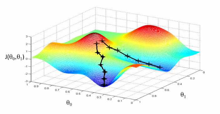
Let’s begin with stochastic gradient descent’s predecessor and cousin: gradient descent. Gradient descent is an algorithm that iteratively tweaks a model’s parameters, with the goal of minimizing the discrepancy between the model’s predictions and the “true” labels associated with a set of training examples.

This discrepancy is commonly termed “cost” or “loss” and is quantified in a cost function. Here’s a common cost function used with gradient descent: $$ \begin{aligned} J(\theta) = \frac{1}{2m} \sum_{i=1}^{m} (h_{\theta}(x^{(i)}) - y^{(i)})^2 \end{aligned} $$

Let’s unpack this. Here \(m\) is the number of training examples, \(x^{(i)}\) is the \(i\)th training example, \(y^{(i)}\) is the \(i\)th corresponding label, and θ is a vector representation of our model’s parameters. So h_θ(x⁽ⁱ⁾) is the prediction our model h_θ makes on example \(x^{(i)}\).

Then (h_θ(x⁽ⁱ⁾) − y⁽ⁱ⁾)² is the square of the difference between our model’s prediction and the actual label for the \(i\)th training example. We sum over all the training examples, and divide by \(m\) to compute the average, squared-error.

So is J(θ) just one-half of the mean-squared error on the training examples.

Note that we could aim to minimize any multiple of the mean-squared error, and we’d still be minimizing the actual mean-squared error in the process. Thus, it’s reasonable to take J(θ) as our particular cost function.

Now back to gradient descent. At each iteration, we perform an update operation on our parameter vector θ. The full algorithm:

    Gradient Descent $$ \begin{aligned} & \text{repeat until convergence } \{ \\ & \quad \theta \leftarrow \theta - \gamma \nabla J(\theta) \\ & \} \end{aligned} $$

Here is γ is the learning rate, or step-size. Recall that ∇J(θ) is the vector derivative of J(θ), and points in the direction in which J(θ) rises most rapidly. So to minimize J(θ), we simply take a step of size γ in the exact opposite direction.

We do this repeatedly until we arrive at a point where ∇J(θ) = 0. This represents a local or global minimum of our cost function J(θ). At such a point, we say gradient descent has converged. Note that if J(θ) has certain properties, notably convexity, and γ is properly tuned, gradient descent will in fact converge at the global minimum.²

To be totally clear, the update operation θ − γ∇J(θ) is a vector subtraction. Both the parameter vector, θ, and the gradient, ∇J(θ), are \(n\)-dimensional vectors, where \(n\) denotes the number of features in our model. So every update operation in gradient descent is performed on the \(n\)-dimensional feature space of our model.

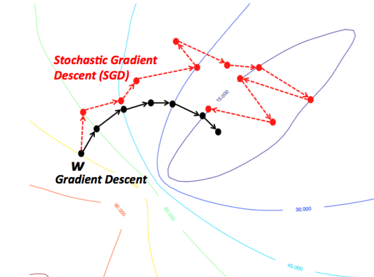
Stochastic Gradient Descent

Gradient descent has a problem. Computing the gradient of the cost function, ∇J(θ), is very costly in practice. Recall $$ \begin{aligned} \nabla J(\theta) = (\frac{\partial}{\partial \theta_1} J(\theta), \frac{\partial}{\partial \theta_2} J(\theta), ..., \frac{\partial}{\partial \theta_n} J(\theta)) \end{aligned} $$

where the subscripts represent an index on features. Each partial derivative in this vector involves computing a sum over every training example: $$ \begin{aligned} \frac{\partial}{\partial \theta_j} J(\theta) &= \frac{\partial}{\partial \theta_j} \left( \frac{1}{2m} \sum_{i=1}^{m} (h_{\theta}(x^{(i)}) - y^{(i)})^2 \right) \\ &= \frac{1}{m} \sum_{i=1}^{m} (h_{\theta}(x^{(i)}) - y^{(i)}) \frac{\partial}{\partial \theta_j} h_{\theta}(x^{(i)}) \end{aligned} $$

(Note that we are using a different index, \(j\), for the partial derivatives, as they are taken with respect to the model’s \(n\) features. The index \(i\) refers to the training examples.)

For large training sets (as most are), this is prohibitively expensive. The key idea in stochastic gradient descent is to drop the sum, and use the following as a very rough proxy for our partial derivative: $$ \begin{aligned} \frac{\partial}{\partial \theta_j} J(\theta) \approx (h_{\theta}(x^{(i)}) - y^{(i)}) \frac{\partial}{\partial \theta_j} h_{\theta}(x^{(i)}) \end{aligned} $$ where (x⁽ⁱ⁾, y⁽ⁱ⁾) is any one particular training example.

Then, in stochastic gradient descent, instead of summing over every training example at each step, and iterating until convergence, we cycle through the training examples in random order, using a single one at each iteration in our cost function:

    Stochastic Gradient Descent $$ \begin{aligned} & \text{repeat until convergence } \{ \\ & \quad \text{for } i := 1, 2, ..., m \space \{ \\ & \quad \quad \theta \leftarrow \theta - \gamma \nabla J(\theta; x^{(i)}; y^{(i)}) \\ & \quad \} \\ & \} \end{aligned} $$

where we have, from above: $$ \begin{aligned} \nabla J(\theta; x^{(i)}; y^{(i)}) = (h_{\theta}(x^{(i)}) - y^{(i)}) \nabla h_{\theta}(x^{(i)}) \end{aligned} $$

Note that, in practice, the number of times we have to run the inner loop depends on the size of the training set. If the number of training examples is huge, a single iteration through the training examples can suffice. Most data sets require between 1 to 10 runs though the inner loop.

Though it may not be immediately obvious, theory assures us that if the learning rate γ is reduced appropriately over time, and the cost function satisfies certain properties (i.e. convexity), stochastic gradient descent will also converge.

Finally, it is worth noting that there is a middle-ground between gradient descent and stochastic gradient descent, called mini-batch gradient descent. Mini-batch gradient descent uses a randomly selected subset, or mini-batch, of \(b\) training examples at each iteration, instead of just one. Some definitions of SGD actually refer to mini-batch gradient descent. In practice, batching can lead to a more stable trajectory than in SGD, and, perhaps surprisingly, better performance as well, given that the gradient computation is properly vectorized.³

Parallelization

Note that stochastic gradient descent, as we have described it thus far, is a sequential algorithm. Each update operation involves both 1) reading the current parameter vector θ, and 2) writing to θ a modified value. So we cannot just naively execute a series of update operations in parallel.

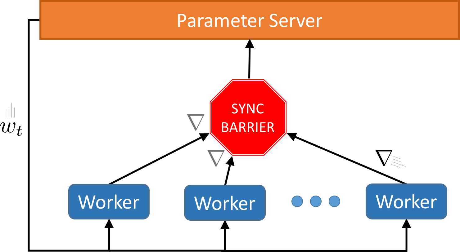
How would we go about parallelizing SGD? One could imagine an approach in which we take snapshot reads of the parameter vector, and periodically merge updates based on a given read in a synchronization step.

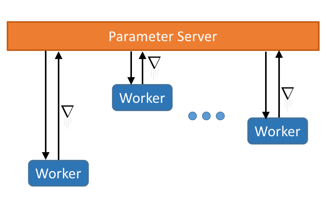
Alternatively, we could get rid of synchronization altogether, and have worker threads (or processes) read the parameter vector from a shared memory bus, compute a gradient, and then send back an update to a master. It would then be the master node’s responsibility to incorporate the updates in some total ordering, while sensibly handling concurrent writes (e.g. via locks).

Is there any guarantee that SGD with version reconciliation would converge? What would be the impact on performance of explicit synchronization (approach 1) and arbitrary locking (approach 2)?

These are the questions that the literature on parallelizing stochastic gradient descent seeks to answer.

Thanks to Kiran Vodrahalli, Prem Nair, and Sanjay Jain for reviewing drafts of this post.

Footnotes

---

1. There is also an important intermediate stage: validation, used to determine the values of our model’s hyperparameters. Hyperparameters are meta-parameters that dictate how a particular model is constructed. In gradient descent, the learning rate γ is a key hyperparameter.↩︎

2. A function is convex if a line segment between any two points on its graph lies above or on the graph. An upward-facing parabola is a simple example of a convex function. The problem of minimizing convex functions, or convex optimization, is an entire subfield of theoretical machine learning. See these slides for a brief proof sketch that gradient descent converges on convex functions.↩︎

3. Assuming the appropriate vectorization libraries are present, it may be possible to compute the following batch gradient in parallel on a multi-core machine: $$ \begin{aligned} \nabla J(B) = \frac{1}{|B|} \sum_{i=1}^{|B|} (h_{\theta}(x^{(i)}) - y^{(i)}) \nabla h_{\theta}(x^{(i)}) \end{aligned} $$ In a recent paper, Facebook AI Research took this idea to the extreme, training ImageNet in 1 hour with a mini-batch size of 8192 images on 256 GPUs.↩︎

---

---